Prediction performance metrics

1. Why use several prediction metrics?

Continuous predictions may be generated using machine-learning algorithms, statistical models, geostatistical methods, or process-based models. modelskill provides tools to evaluate the agreement between paired observations and predictions using a range of complementary performance metrics.

Predictive performance is inherently multidimensional. A model may exhibit low overall error while retaining systematic bias, reproduce the observed pattern while consistently over- or underpredicting, or achieve good aggregate accuracy while failing to capture the observed variability.

Accordingly, model evaluation should generally rely on a combination of complementary metrics rather than a single summary statistic, so that different aspects of predictive performance can be assessed explicitly.

Performance metrics should be computed using independent validation data whenever possible, or using an appropriate resampling or cross-validation procedure when an independent validation dataset is not available.

2. Example data

We create three deliberately different prediction models.

library(modelskill)

set.seed(123)

n <- 100

obs <- seq(0, 10, length.out = n) +
  rnorm(n, sd = 1)

models <- list(
  Good = obs + rnorm(n, sd = 0.5),

  # Constant positive offset
  Biased = obs + 1,

  # Larger random errors
  Noisy = obs + rnorm(n, sd = 2)
)

The models have simple characteristics:

Good has relatively small random errors;
Biased systematically overpredicts by one unit;
Noisy has larger random errors.

3. Start by looking at the predictions

Before calculating summary statistics, it is useful to inspect observed versus predicted values.

plot_data <- data.frame(
  observed = rep(obs, times = length(models)),
  predicted = unlist(models, use.names = FALSE),
  model = rep(names(models), each = length(obs))
)

ggplot2::ggplot(
  plot_data,
  ggplot2::aes(
    x = observed,
    y = predicted,
    colour = model
  )
) +
  ggplot2::geom_abline(
    slope = 1,
    intercept = 0,
    linetype = "dashed"
  ) +
  ggplot2::geom_point(
    alpha = 0.7,
    size = 1.5
  ) +
  ggplot2::coord_equal() +
  ggplot2::theme_classic() +
  ggplot2::labs(
    x = "Observed",
    y = "Predicted",
    colour = "Model"
  )

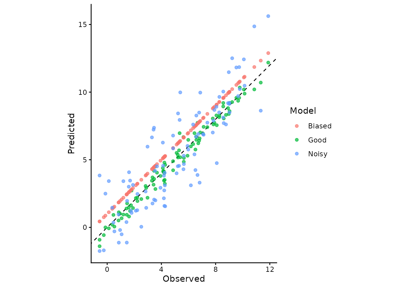
The dashed 1:1 line represents perfect agreement. Good remains relatively close to this line, Biased is systematically shifted upward, and Noisy is more dispersed.

4. Calculate individual metrics

Every prediction metric in modelskill can be calculated separately. This is useful when only a few specific aspects of performance are required.

All individual functions use the same basic argument order:

metric(obs, pred)

where obs is the vector of observations and pred is the corresponding prediction vector.

4.1 RMSE: overall error magnitude

The root mean squared error (RMSE) measures the overall magnitude of prediction errors:

\mathrm{RMSE} = \sqrt{ \frac{1}{n} \sum_{i=1}^{n} (obs_i-pred_i)^2 }.

Calculate RMSE for the Good model:

rmse(
  obs,
  models$Good
)
#> [1] 0.4840658

and compare it with the Noisy model:

rmse(
  obs,
  models$Noisy
)
#> [1] 1.905528

rmse() is non-negative and has the same units as the response variable. Zero indicates perfect predictions and smaller values indicate smaller errors.

Because errors are squared before averaging, relatively large errors have more influence on RMSE. It is therefore useful to interpret RMSE together with a less outlier-sensitive statistic such as mae().

rmse(obs, models$Noisy)
#> [1] 1.905528
mae(obs, models$Noisy)
#> [1] 1.513235

4.2 Bias: systematic overprediction or underprediction

modelskill defines prediction error as

e_i = obs_i-pred_i.

The bias() function calculates the mean signed error:

\mathrm{ME} = \frac{1}{n} \sum_{i=1}^{n} (obs_i-pred_i).

For the deliberately biased model:

bias(
  obs,
  models$Biased
)
#> [1] -1

Because Biased = obs + 1, its mean error is -1.

Under the modelskill convention:

negative bias means overprediction;
positive bias means underprediction;
zero bias means no average systematic error.

A bias close to zero does not necessarily mean that predictions are accurate. Positive and negative errors can cancel. Bias should therefore be interpreted with an unsigned error metric such as MAE or RMSE.

5. A particularly important distinction: `r2()` versus `R2()`

modelskill contains two statistics whose names differ only by capitalization, but they measure different things.

5.1 Lowercase `r2()`

r2() is squared Pearson correlation:

r^2 = \left[ \frac{ \sum_{i=1}^{n} (obs_i-\bar{obs})(pred_i-\bar{pred}) }{ \sqrt{ \sum_{i=1}^{n}(obs_i-\bar{obs})^2 \sum_{i=1}^{n}(pred_i-\bar{pred})^2 } } \right]^2.

It measures the strength of linear association.

5.2 Uppercase `R2()`

R2() is the model-efficiency coefficient:

R^2 = 1- \frac{ \sum_{i=1}^{n}(obs_i-pred_i)^2 }{ \sum_{i=1}^{n}(obs_i-\bar{obs})^2 }.

It compares the model with using the observed mean as a constant prediction.

This distinction becomes obvious with the Biased model:

r2(
  obs,
  models$Biased
)
#> [1] 1

R2(
  obs,
  models$Biased
)
#> [1] 0.8974284

The biased predictions are exactly one unit above the observations. Their linear association is therefore perfect, so lowercase r2() is 1.

However, the predictions are not perfectly accurate. Uppercase R2() detects their prediction error and is therefore below 1.

This illustrates why correlation and squared correlation should not be used alone as measures of prediction accuracy.

Remember: lowercase r2() is squared Pearson correlation. Uppercase R2() is model efficiency.

In modelskill, uppercase R2(), nse(), and mec() are aliases for exactly the same statistic:

c(
  R2 = R2(obs, models$Good),
  NSE = nse(obs, models$Good),
  MEC = mec(obs, models$Good)
)
#>        R2       NSE       MEC 
#> 0.9759654 0.9759654 0.9759654

For this statistic:

1 is perfect prediction;
0 means that predicting the observed mean performs equally well;
negative values mean that predicting the observed mean would perform better.

The distinction between r^2 and R^2 (also referred to as NSE or MEC) has been highlighted on many occasions (e.g., Legates and McCabe 1999; Wadoux et al. 2022). It is also discussed on the Wikipedia page on the coefficient of determination, which notes that r^2 quantifies the strength of the linear relationship between observed and predicted values, whereas evaluation of predictive goodness-of-fit should concern the specific 1:1 relationship,

obs = 1 \times pred + 0.

A high r^2 can therefore occur even when predictions are systematically biased or otherwise depart substantially from the 1:1 line.

5.3 Correlation is not agreement

The same issue can be illustrated by comparing Pearson correlation with Lin’s concordance correlation coefficient.

correlation(
  obs,
  models$Biased
)
#> [1] 1

ccc(
  obs,
  models$Biased
)
#> [1] 0.9512161

correlation() measures linear association. It is insensitive to a constant shift.

ccc() measures concordance and is reduced when predictions differ from observations in their mean or variability. It therefore measures agreement more directly than Pearson correlation.

6. Compare several models at once

When several models are being evaluated, model_metrics() calculates the main prediction metrics together.

model_metrics(
  models,
  obs,
  digits = 3
)
#>         model   bias   mae   mse  rmse nrmse crmse correlation    r2    R2
#> Good     Good  0.054 0.382 0.234 0.484 0.154 0.481       0.989 0.977 0.976
#> Biased Biased -1.000 1.000 1.000 1.000 0.319 0.000       1.000 1.000 0.897
#> Noisy   Noisy -0.241 1.513 3.631 1.906 0.607 1.890       0.866 0.749 0.628
#>        sd_ratio   ccc    Cb
#> Good      1.023 0.988 1.000
#> Biased    1.000 0.951 0.951
#> Noisy     1.206 0.849 0.980

The default output contains complementary information about:

systematic error;
average error magnitude;
centred error;
association;
model efficiency;
variability;
concordance.

For the example data, no single column should be used to identify the “best” model without considering what aspect of prediction quality matters for the application.

7. Categories of prediction performance metrics

The following classification is intended as a practical guide. Some metrics are mathematically related and should not be interpreted as independent evidence.

Category	`modelskill` functions	Main question
Systematic error	`bias()`, `mpe()`	Are predictions systematically too high or too low?
Error magnitude	`mae()`, `mdae()`, `mse()`, `rmse()`	How large are the prediction errors?
Centred error and spread	`crmse()`, `sep()`, `sd_ratio()`	How much disagreement remains after bias is removed, and is variability reproduced?
Association	`correlation()`, `r2()`	Do predictions reproduce the observed pattern?
Agreement	`ccc()`, `willmott_d()`	How closely do predicted values agree with observations?
Efficiency and benchmark performance	`R2()`, `nse()`, `mec()`, `rae()`, `kge()`	How well does the model perform relative to a benchmark or multiple performance components?
Scaled and relative error	`nrmse()`, `rrmse()`, `rpd()`, `rpiq()`, `rer()`	How large is error relative to the scale or variability of the observations?
Relative and transformed losses	`mape()`, `smape()`, `msle()`, `rmsle()`	How large is error on a relative or logarithmic scale?
Quantile loss	`pinball_loss()`	How accurate is a prediction for a specified quantile?

There is no universally best metric. The appropriate combination depends on the scientific objective and the consequences of different types of prediction error.

8. Core metrics

The default output of model_metrics() contains the principal metrics used for continuous prediction evaluation.

For the retained observation-prediction pairs, let o_i denote observations, p_i predictions, and n the number of pairs. Let \bar{o} and \bar{p} denote their means.

Metric / function	Equation	Ideal	Simple interpretation	Reference
ME / bias `bias()`	\mathrm{ME}=\frac{1}{n}\sum_i(o_i-p_i)	0	Average signed error. Negative = overprediction; positive = underprediction.	(Legates and McCabe 1999)
MAE `mae()`	\mathrm{MAE}=\frac{1}{n}\sum_i\lvert o_i-p_i\rvert	0	Average absolute error in response units.	(Willmott and Matsuura 2005)
MSE `mse()`	\mathrm{MSE}=\frac{1}{n}\sum_i(o_i-p_i)^2	0	Average squared error; gives more weight to large errors.	(Hodson 2022)
RMSE `rmse()`	\mathrm{RMSE}=\sqrt{\frac{1}{n}\sum_i(o_i-p_i)^2}	0	Overall error magnitude in response units; sensitive to large errors.	(Hodson 2022)
NRMSE `nrmse()`	\mathrm{NRMSE}=\mathrm{RMSE}/s_o	0	RMSE relative to the observed standard deviation.	(Taylor 2001)
cRMSE `crmse()`	\mathrm{cRMSE}=\sqrt{\frac{1}{n}\sum_i[(o_i-p_i)-\mathrm{ME}]^2}	0	Error remaining after mean bias is removed.	(Taylor 2001)
Pearson correlation `correlation()`	r=\frac{\sum_i(o_i-\bar{o})(p_i-\bar{p})}{\sqrt{\sum_i(o_i-\bar{o})^2\sum_i(p_i-\bar{p})^2}}	1	Strength and direction of linear association; not agreement.	(Legates and McCabe 1999)
Squared Pearson correlation `r2()`	r^2 = r^2	1	Strength of linear association without its sign; not agreement.	(Legates and McCabe 1999)
Model efficiency R^2 `R2()`	R^2 = 1-\frac{\sum_i(o_i-p_i)^2}{\sum_i(o_i-\bar{o})^2}	1	1 = perfect; 0 = no better than predicting the observed mean; negative = worse than predicting the observed mean.	(Nash and Sutcliffe 1970; Janssen and Heuberger 1995)
SD ratio `sd_ratio()`	\mathrm{SD\ ratio} = \frac{s_p}{s_o}	1	Below 1 = too little variability; above 1 = too much variability.	(Taylor 2001)
CCC `ccc()`	\mathrm{CCC} = \frac{2c_{op}}{v_o+v_p+(\bar{o}-\bar{p})^2}	1	Agreement in correlation, mean, and variability.	(Lin 1989)
Bias correction factor C_b `model_metrics()`	C_b = \frac{2\sqrt{v_ov_p}}{v_o+v_p+(\bar{o}-\bar{p})^2}	1	Agreement in mean and variability, without correlation.	(Lin 1989)

Here s_o and s_p are the sample standard deviations of observations and predictions. For CCC, v_o, v_p, and c_{op} are the corresponding population variances and covariance used by the package.

The ranges and special cases of each metric are described in its linked reference page.

9. Extended metrics

Additional metrics are available when a more specialised evaluation is required.

model_metrics(
  models,
  obs,
  extended = TRUE,
  digits = 3
)
#>         model   bias   mae   mse  rmse nrmse crmse correlation    r2    R2
#> Good     Good  0.054 0.382 0.234 0.484 0.154 0.481       0.989 0.977 0.976
#> Biased Biased -1.000 1.000 1.000 1.000 0.319 0.000       1.000 1.000 0.897
#> Noisy   Noisy -0.241 1.513 3.631 1.906 0.607 1.890       0.866 0.749 0.628
#>        sd_ratio   ccc    Cb  mdae   rpd   rpiq   sep    rer    mape     mpe
#> Good      1.023 0.988 1.000 0.312 6.483 11.063 0.483 25.709  17.597   1.271
#> Biased    1.000 0.951 0.951 1.000 3.138  5.355 0.000 12.445  55.918 -25.264
#> Noisy     1.206 0.849 0.980 1.213 1.647  2.810 1.900  6.531 105.193  -7.746
#>         smape msle rmsle   rae  rrmse willmott_d   kge
#> Good   18.659   NA    NA 0.144  9.509      0.994 0.972
#> Biased 33.766   NA    NA 0.377 19.645      0.975 0.804
#> Noisy  49.121   NA    NA 0.570 37.434      0.920 0.750

The extended output adds robust error measures, scale-normalised metrics, percentage errors, agreement measures, and KGE (2009).

These metrics should be selected because they answer a relevant scientific question, not simply because they are available.

For example, the median absolute error is less affected by a few unusually large errors than RMSE:

mdae(
  obs,
  models$Noisy
)
#> [1] 1.212603

KGE (2009), the original Kling-Gupta efficiency formulation, combines correlation, variability, and mean agreement:

kge(
  obs,
  models$Good
)
#> [1] 0.9720975

9.1 Extended metric reference

Metric / function	Equation	Ideal	Simple interpretation	Reference
MdAE `mdae()`	\mathrm{MdAE} = \mathrm{median}_i\lvert o_i-p_i\rvert	0	Typical absolute error; relatively robust to large errors.	(Hyndman and Koehler 2006)
RPD `rpd()`	\mathrm{RPD} = s_o/\mathrm{RMSE}	Larger	Error relative to observed standard deviation.	(Bellon-Maurel et al. 2010)
RPIQ `rpiq()`	\mathrm{RPIQ} = \mathrm{IQR}(o)/\mathrm{RMSE}	Larger	Error relative to the observed interquartile range.	(Bellon-Maurel et al. 2010)
SEP `sep()`	\mathrm{SEP} = \sqrt{\frac{1}{n-1}\sum_i[(o_i-p_i)-\mathrm{ME}]^2}	0	Sample SD of prediction errors after removing bias.	(Bellon-Maurel et al. 2010)
RER `rer()`	\mathrm{RER} = \frac{\max(o)-\min(o)}{\mathrm{RMSE}}	Larger	Error relative to observed range; sensitive to extreme values.	(Bellon-Maurel et al. 2010)
MAPE `mape()`	\mathrm{MAPE} = \frac{100}{n}\sum_i\left\lvert\frac{o_i-p_i}{o_i}\right\rvert	0	Mean absolute percentage error. Undefined when an observation is zero.	(Hyndman and Koehler 2006)
MPE `mpe()`	\mathrm{MPE} = \frac{100}{n}\sum_i\frac{o_i-p_i}{o_i}	0	Signed relative bias in percent. Undefined when an observation is zero.	(Hyndman and Koehler 2006)
sMAPE `smape()`	\mathrm{sMAPE} = \frac{100}{n}\sum_i\frac{2\lvert o_i-p_i\rvert}{\lvert o_i\rvert+\lvert p_i\rvert}	0	Symmetric absolute percentage error (0–200%).	(Hyndman and Koehler 2006)
MSLE `msle()`	\mathrm{MSLE} = \frac{1}{n}\sum_i[\log(1+o_i)-\log(1+p_i)]^2	0	Squared error on the log1p scale. Requires non-negative values.	(Hodson 2022)
RMSLE `rmsle()`	\mathrm{RMSLE} = \sqrt{\mathrm{MSLE}}	0	Root mean squared error on the log1p scale.	(Hodson 2022)
RAE `rae()`	\mathrm{RAE} = \frac{\sum_i\lvert o_i-p_i\rvert}{\sum_i\lvert o_i-\bar{o}\rvert}	0	Absolute error relative to predicting the observed mean; 1 is the benchmark.	(Hyndman and Koehler 2006)
RRMSE `rrmse()`	\mathrm{RRMSE} = 100\,\mathrm{RMSE}/\lvert\bar{o}\rvert	0	RMSE as a percentage of the absolute observed mean.	(Willmott et al. 1985)
Willmott’s d `willmott_d()`	d = 1-\frac{\sum_i(o_i-p_i)^2}{\sum_i(\lvert p_i-\bar{o}\rvert+\lvert o_i-\bar{o}\rvert)^2}	1	Index of agreement; sensitive to large errors.	(Willmott et al. 1985)
KGE (2009) `kge()`	\mathrm{KGE} = 1-\sqrt{(r-1)^2+(s_p/s_o-1)^2+(\bar{p}/\bar{o}-1)^2}	1	Combines correlation, variability ratio, and mean ratio.	(Gupta et al. 2009)

MAPE, MPE, sMAPE, and RRMSE are returned as percentages. sMAPE ranges from 0 to 200%; the other percentage metrics are unbounded above.

Percentage-based metrics require particular care when observations or their mean are zero or close to zero.

10. Quantile predictions

pinball_loss() is not included in model_metrics(extended = TRUE) because it requires a specific quantile level.

For a quantile prediction q_\tau, the loss depends on the requested probability \tau.

For example, at the median:

pinball_loss(
  obs,
  models$Good,
  level = 0.5
)
#> [1] 0.1910524

At level = 0.5, pinball loss is one-half of MAE.

For a 90th-percentile prediction:

pinball_loss(
  obs,
  predicted_q90,
  level = 0.90
)

The quantile level should be chosen according to the prediction being evaluated.

11. How should metrics be combined?

A useful general-purpose evaluation of continuous predictions should usually contain metrics from different categories.

For example:

data.frame(
  bias = bias(obs, models$Good),
  mae = mae(obs, models$Good),
  rmse = rmse(obs, models$Good),
  correlation = correlation(obs, models$Good),
  R2 = R2(obs, models$Good),
  ccc = ccc(obs, models$Good)
)
#>        bias       mae      rmse correlation        R2     ccc
#> 1 0.0537734 0.3821047 0.4840658   0.9886633 0.9759654 0.98826

This combination answers several distinct questions:

bias() — is there systematic overprediction or underprediction?
mae() — what is the typical absolute error?
rmse() — what is the squared-error-weighted error magnitude?
correlation() — is the observed pattern reproduced?
R2() — does the model outperform the observed-mean benchmark?
ccc() — how closely do predicted values agree with observations overall?

The precise set should depend on the application. There is no universal threshold at which RMSE, correlation, CCC, KGE (2009), or another metric automatically becomes “good”.

Several available statistics are mathematically related.

For example:

\mathrm{MSE}=\mathrm{RMSE}^2,

and, when defined,

\mathrm{RPD} = \frac{1}{\mathrm{NRMSE}}.

SEP and cRMSE also contain essentially the same centred error information but use different divisors.

Similarly, R2(), nse(), and mec() are three names for exactly the same statistic in modelskill.

These functions remain available because different scientific communities use different conventions, but reporting several mathematically equivalent metrics does not provide independent evidence about model performance.

13. Missing values and special cases

By default, modelskill removes incomplete observation-prediction pairs separately for each model.

For example:

obs_missing <- obs
pred_missing <- models$Good

pred_missing[c(5, 20)] <- NA

rmse(
  obs_missing,
  pred_missing
)
#> [1] 0.4838553

For fair comparison among several models, it is generally preferable that all models are evaluated on the same validation observations.

Some metrics are undefined in particular situations:

Pearson correlation and r2() are undefined for constant vectors;
R2() / NSE / MEC are undefined when the observations are constant;
percentage metrics can be undefined or unstable when their denominators are zero or close to zero;
MSLE and RMSLE require non-negative observations and predictions;
KGE (2009) requires variation in both observations and predictions and a non-zero observed mean.

The individual function documentation describes these cases in detail.

14. Practical recommendations

For most prediction-validation analyses:

Inspect observations versus predictions first.
Summary metrics can hide structure visible in the raw comparison.
Report error magnitude.
MAE and/or RMSE provide interpretable error measures in response units.
Report systematic error.
Bias indicates whether predictions are systematically too high or too low.
Separate association from accuracy.
Correlation and lowercase r2() measure association and can remain high despite substantial prediction bias.
Use an agreement or efficiency measure when useful.
CCC measures agreement, while uppercase R2() / NSE / MEC compares model performance with the observed-mean benchmark.
Use specialised metrics only when their interpretation fits the problem.
Percentage errors, RPD, RPIQ, KGE (2009), and quantile loss can be useful, but should not automatically be reported for every application.
Do not select a model from one metric alone.
Different metrics describe different aspects of prediction quality.

15. References

Bellon-Maurel, V., Fernandez-Ahumada, E., Palagos, B., Roger, J.-M., and McBratney, A. (2010). Critical review of chemometric indicators commonly used for assessing the quality of the prediction of soil attributes by NIR spectroscopy. Trends in Analytical Chemistry, 29, 1073-1081. https://doi.org/10.1016/j.trac.2010.05.006
Gupta, H. V., Kling, H., Yilmaz, K. K., and Martinez, G. F. (2009). Decomposition of the mean squared error and NSE performance criteria: implications for improving hydrological modelling. Journal of Hydrology, 377, 80-91. https://doi.org/10.1016/j.jhydrol.2009.08.003
Hodson, T. O. (2022). Root-mean-square error (RMSE) or mean absolute error (MAE): when to use them or not. Geoscientific Model Development, 15, 5481-5487. https://doi.org/10.5194/gmd-15-5481-2022
Hyndman, R. J. and Koehler, A. B. (2006). Another look at measures of forecast accuracy. International Journal of Forecasting, 22, 679-688. https://doi.org/10.1016/j.ijforecast.2006.03.001
Janssen, P. H. M. and Heuberger, P. S. C. (1995). Calibration of process-oriented models. Ecological Modelling, 83, 55-66. https://doi.org/10.1016/0304-3800(95)00084-9
Koenker, R. and Bassett, G. (1978). Regression quantiles. Econometrica, 46, 33-50. https://doi.org/10.2307/1913643
Legates, D. R. and McCabe, G. J. (1999). Evaluating the use of goodness-of-fit measures in hydrologic and hydroclimatic model validation. Water Resources Research, 35, 233-241. https://doi.org/10.1029/1998WR900018
Lin, L. I.-K. (1989). A concordance correlation coefficient to evaluate reproducibility. Biometrics, 45, 255-268. https://doi.org/10.2307/2532051
Nash, J. E. and Sutcliffe, J. V. (1970). River flow forecasting through conceptual models part I: A discussion of principles. Journal of Hydrology, 10, 282-290. https://doi.org/10.1016/0022-1694(70)90255-6
Taylor, K. E. (2001). Summarizing multiple aspects of model performance in a single diagram. Journal of Geophysical Research, 106, 7183-7192. https://doi.org/10.1029/2000JD900719
Willmott, C. J., Ackleson, S. G., Davis, R. E., Feddema, J. J., Klink, K. M., Legates, D. R., O’Donnell, J., and Rowe, C. M. (1985). Statistics for the evaluation and comparison of models. Journal of Geophysical Research, 90, 8995-9005. https://doi.org/10.1029/JC090iC05p08995
Willmott, C. J. and Matsuura, K. (2005). Advantages of the mean absolute error (MAE) over the root mean square error (RMSE) in assessing average model performance. Climate Research, 30, 79-82. https://doi.org/10.3354/cr030079

16. Next steps

Use the predictive-uncertainty evaluation article when models provide prediction intervals, quantiles, standard deviations, or complete predictive distributions.

Use the summary diagrams and diagnostic plots article to compare several models graphically using solar, target, and Taylor diagrams.

Bellon-Maurel, Veronique, Elena Fernandez-Ahumada, Benoit Palagos, Jean-Michel Roger, and Alex McBratney. 2010. “Critical Review of Chemometric Indicators Commonly Used for Assessing the Quality of the Prediction of Soil Attributes by NIR Spectroscopy.” Trends in Analytical Chemistry 29: 1073–81. https://doi.org/10.1016/j.trac.2010.05.006.

Gupta, Hoshin V., Harald Kling, Koray K. Yilmaz, and Guillermo F. Martinez. 2009. “Decomposition of the Mean Squared Error and NSE Performance Criteria: Implications for Improving Hydrological Modelling.” Journal of Hydrology 377: 80–91. https://doi.org/10.1016/j.jhydrol.2009.08.003.

Hodson, Tim O. 2022. “Root-Mean-Square Error (RMSE) or Mean Absolute Error (MAE): When to Use Them or Not.” Geoscientific Model Development 15: 5481–87. https://doi.org/10.5194/gmd-15-5481-2022.

Hyndman, Rob J., and Anne B. Koehler. 2006. “Another Look at Measures of Forecast Accuracy.” International Journal of Forecasting 22: 679–88. https://doi.org/10.1016/j.ijforecast.2006.03.001.

Janssen, Peter H. M., and Peter S. C. Heuberger. 1995. “Calibration of Process-Oriented Models.” Ecological Modelling 83: 55–66. https://doi.org/10.1016/0304-3800(95)00084-9.

Legates, David R., and Gregory J. McCabe. 1999. “Evaluating the Use of ‘Goodness-of-Fit’ Measures in Hydrologic and Hydroclimatic Model Validation.” Water Resources Research 35: 233–41. https://doi.org/10.1029/1998WR900018.

Lin, Lawrence I.-K. 1989. “A Concordance Correlation Coefficient to Evaluate Reproducibility.” Biometrics 45: 255–68. https://doi.org/10.2307/2532051.

Nash, J. E., and J. V. Sutcliffe. 1970. “River Flow Forecasting Through Conceptual Models Part I—a Discussion of Principles.” Journal of Hydrology 10: 282–90. https://doi.org/10.1016/0022-1694(70)90255-6.

Taylor, Karl E. 2001. “Summarizing Multiple Aspects of Model Performance in a Single Diagram.” Journal of Geophysical Research: Atmospheres 106: 7183–92. https://doi.org/10.1029/2000JD900719.

Wadoux, Alexandre M. J.-C., Dennis J. J. Walvoort, and Dick J. Brus. 2022. “An Integrated Approach for the Evaluation of Quantitative Soil Maps Through Taylor and Solar Diagrams.” Geoderma 405: 115332. https://doi.org/10.1016/j.geoderma.2021.115332.

Willmott, Cort J., Steven G. Ackleson, Robert E. Davis, et al. 1985. “Statistics for the Evaluation and Comparison of Models.” Journal of Geophysical Research 90: 8995–9005. https://doi.org/10.1029/JC090iC05p08995.

Willmott, Cort J., and Kenji Matsuura. 2005. “Advantages of the Mean Absolute Error (MAE) over the Root Mean Square Error (RMSE) in Assessing Average Model Performance.” Climate Research 30: 79–82. https://doi.org/10.3354/cr030079.

Alexandre M.J.-C. Wadoux

1. Why use several prediction metrics?

2. Example data

3. Start by looking at the predictions

4. Calculate individual metrics

4.1 RMSE: overall error magnitude

4.2 Bias: systematic overprediction or underprediction

5. A particularly important distinction: r2() versus R2()

5.1 Lowercase r2()

5.2 Uppercase R2()

5.3 Correlation is not agreement

6. Compare several models at once

7. Categories of prediction performance metrics

8. Core metrics

9. Extended metrics

9.1 Extended metric reference

10. Quantile predictions

11. How should metrics be combined?

12. Related and redundant metrics

13. Missing values and special cases

14. Practical recommendations

15. References

16. Next steps

5. A particularly important distinction: `r2()` versus `R2()`

5.1 Lowercase `r2()`

5.2 Uppercase `R2()`