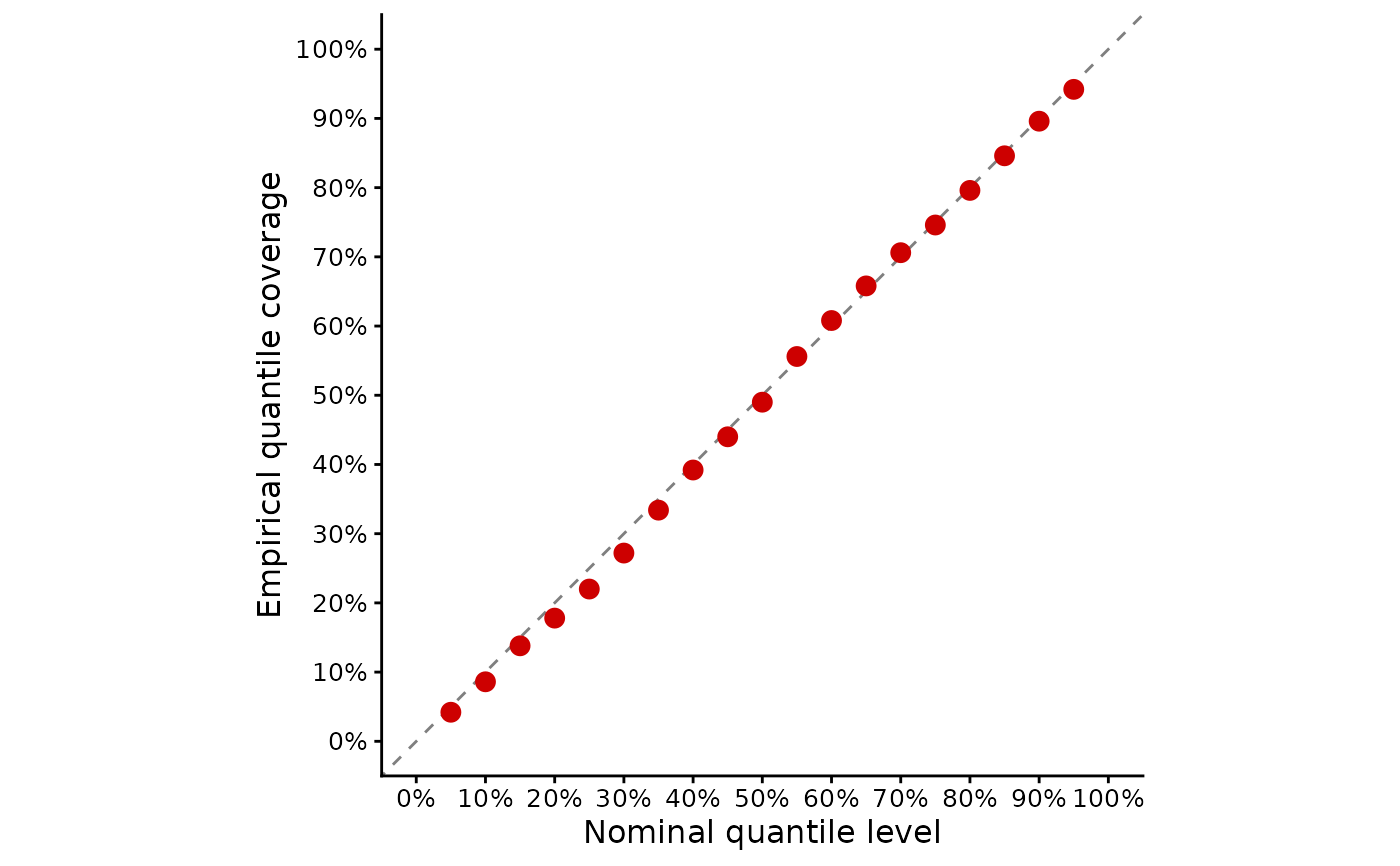
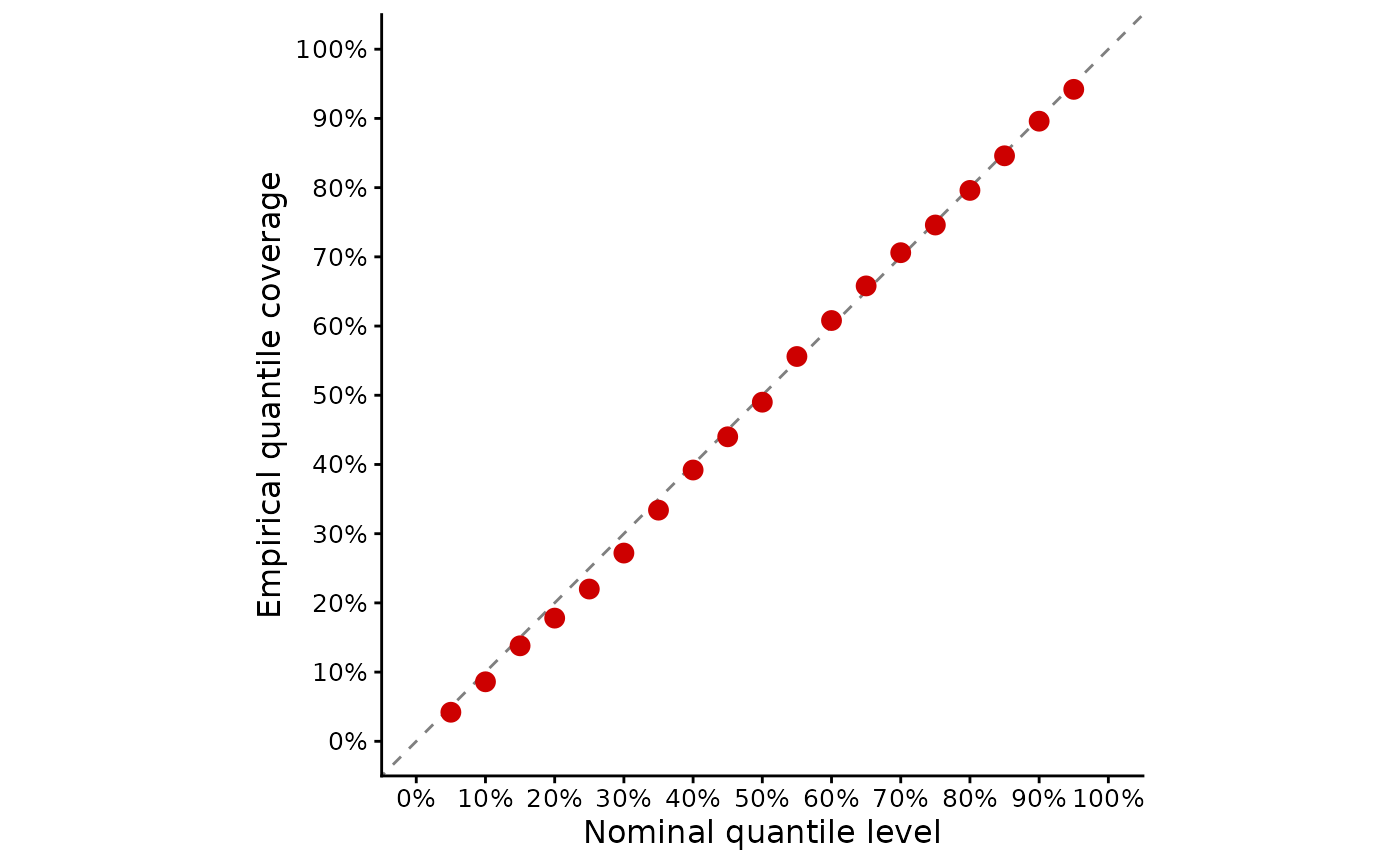
Plots empirical quantile coverage probability (QCP) against the corresponding
nominal predictive quantile levels. For a calibrated predictive distribution,
approximately a proportion p of observations should fall below the predicted
p-quantile. Points should therefore follow the dashed 1:1 line.
Usage
gg_qcp(
  obs,
  quantiles = NULL,
  levels = NULL,
  pred = NULL,
  predictive_sd = NULL,
  na.rm = TRUE,
  point_size = 3,
  distribution = NULL
)
Arguments
- obs
Numeric observation vector.
- quantiles
Numeric matrix or data frame containing predicted quantiles in columns. Required unless
predandpredictive_sd, ordistribution, are supplied.- levels
Numeric vector of nominal quantile probabilities corresponding to the columns of
quantiles. With predictive means and standard deviations or predictive samples, defaults toseq(0.05, 0.95, by = 0.05).- pred
Optional numeric vector of predictive means. Must be supplied together with
predictive_sd; in this mode predictive quantiles are generated assuming normal predictive distributions.- predictive_sd
Optional numeric vector of predictive standard deviations. Must be supplied together with
pred.- na.rm
Logical; remove incomplete observation/quantile rows?
- point_size
Positive numeric point size.
- distribution
Optional numeric matrix or data frame of equally weighted predictive samples: one row per observation and one column per predictive draw. Supply this instead of bounds or predictive means and standard deviations. At least one draw is required; infinite values are not allowed.
Details
Unlike gg_coverage(), which evaluates the joint coverage of central
prediction intervals, gg_qcp() evaluates individual predictive quantiles.
It can therefore reveal asymmetric or one-sided miscalibration that may be
hidden when lower and upper prediction-interval bounds are assessed together.
Quantiles can be supplied directly through quantiles and levels. When the
predictive distribution is assumed to be normal, they can instead be generated
automatically from predictive means (pred) and predictive standard deviations
(predictive_sd). In this mode, the default is to evaluate quantiles from 0.05
to 0.95 in increments of 0.05.
Predictive samples (distribution) are also accepted, using empirical
quantiles (stats::quantile(), type = 7) at the same default levels.
Supply exactly one representation. As in qcp(), every level uses the same
complete rows across obs and all supplied predictive values. With
na.rm = FALSE, any incomplete row makes coverage missing at every level.
A calibration curve is generally most informative when quantiles are available over a reasonably dense range of probability levels. A smaller number of levels remains valid when only selected predictive quantiles are available.
Examples
set.seed(123)
n <- 500
pred <- seq(0, 10, length.out = n)
predictive_sd <- rep(1, n)
obs <- stats::rnorm(n, mean = pred, sd = predictive_sd)
# Generate a quantile-calibration curve directly from a normal
# predictive distribution
gg_qcp(
obs,
pred = pred,
predictive_sd = predictive_sd
)
 # Predicted quantiles can also be supplied directly
levels <- seq(0.05, 0.95, by = 0.05)
quantiles <- vapply(
levels,
function(p) pred + stats::qnorm(p) * predictive_sd,
numeric(n)
)
gg_qcp(
obs,
quantiles = quantiles,
levels = levels
)
# Predicted quantiles can also be supplied directly
levels <- seq(0.05, 0.95, by = 0.05)
quantiles <- vapply(
levels,
function(p) pred + stats::qnorm(p) * predictive_sd,
numeric(n)
)
gg_qcp(
obs,
quantiles = quantiles,
levels = levels
)
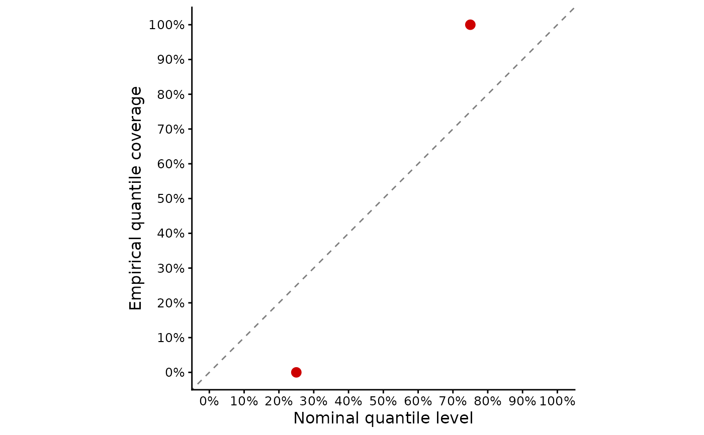
 gg_qcp(1:3, distribution = cbind(0:2, 1:3, 2:4), levels = c(0.25, 0.75))