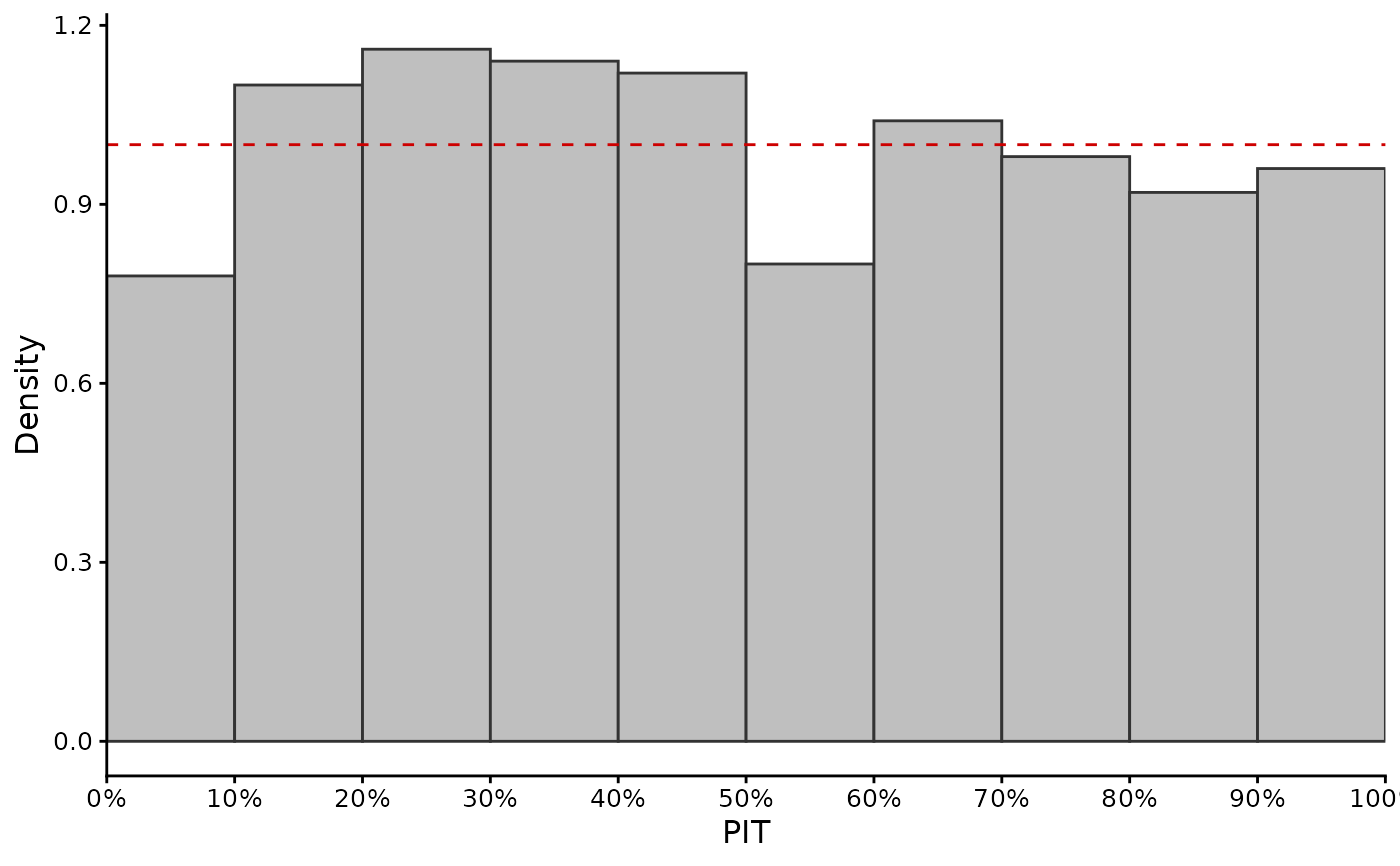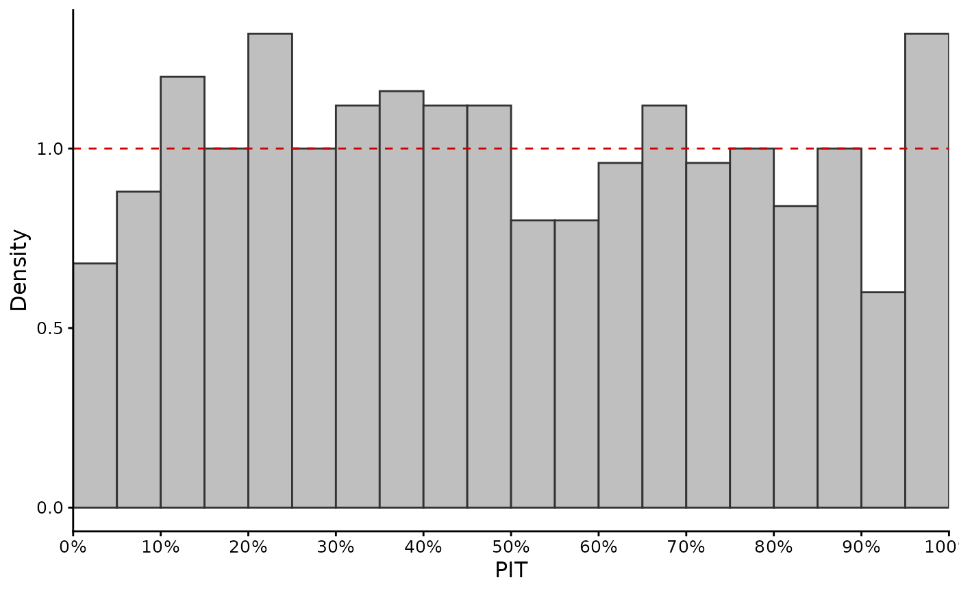
Produces a probability integral transform (PIT) histogram for assessing the calibration of continuous predictive distributions.
Arguments
- pit_values
Numeric vector of PIT values between zero and one, typically calculated with
pit().- bins
Positive integer number of equal-width histogram bins.
- na.rm
Logical; remove missing PIT values? The default is
TRUE.
Value
A ggplot2 object showing the empirical PIT density. Under uniform
calibration the expected density is one.
Details
For observation \(y_i\) with predictive cumulative distribution function \(F_i\), the PIT value is
$$ u_i = F_i(y_i). $$
If the predictive distributions are calibrated and continuous, the PIT values should be approximately uniformly distributed between zero and one. The dashed horizontal line shows the density expected under a uniform distribution.
Departures from uniformity can indicate systematic miscalibration. Common patterns include:
a U-shaped histogram, with excess values near zero and one, which is commonly associated with predictive distributions that are too narrow (underdispersed);
a hump-shaped histogram, with excess values near 0.5, which is commonly associated with predictive distributions that are too wide (overdispersed);
an excess of PIT values near zero, which can occur when predictions are systematically too high relative to the observations;
an excess of PIT values near one, which can occur when predictions are systematically too low relative to the observations.
These patterns are diagnostic rather than unique: different forms of misspecification can produce similar PIT histograms. The PIT should therefore be interpreted together with other calibration and performance diagnostics.
PIT histograms assess the calibration of the complete predictive
distribution. This differs from gg_coverage(), which evaluates central
prediction-interval coverage, and gg_qcp(), which evaluates calibration of
individual predictive quantiles.
The number of histogram bins affects the appearance of the diagnostic. Too few bins may conceal departures from uniformity, whereas too many bins can make sampling variability appear as structure, particularly for small validation datasets.
References
Gneiting, T., Balabdaoui, F. and Raftery, A. E. (2007). Probabilistic forecasts, calibration and sharpness. Journal of the Royal Statistical Society: Series B, 69, 243-268. doi:10.1111/j.1467-9868.2007.00587.x
Schmidinger, J. and Heuvelink, G. B. M. (2023). Validation of uncertainty predictions in digital soil mapping. Geoderma, 437, 116585. doi:10.1016/j.geoderma.2023.116585