Probability integral transform

Calculates probability integral transform (PIT) values for continuous predictive distributions. PIT values can either be supplied directly as predictive cumulative distribution function (CDF) values evaluated at the observations, or calculated from predictive means and standard deviations under a normal predictive-distribution assumption. Predictive samples may instead be supplied through distribution.

Usage

pit(
  cdf_at_obs = NULL,
  obs = NULL,
  pred = NULL,
  predictive_sd = NULL,
  na.rm = TRUE,
  distribution = NULL
)

Arguments

cdf_at_obs: Optional numeric vector containing predictive CDF values evaluated at the corresponding observations. Values must lie between zero and one. Do not supply this together with obs, pred, or predictive_sd, or distribution.
obs: Optional numeric vector of observations. Must be supplied together with pred and predictive_sd, or with distribution.
pred: Optional numeric vector of predictive means. Used with obs and predictive_sd to calculate PIT values assuming normal predictive distributions.
predictive_sd: Optional numeric vector of predictive standard deviations. Values must be finite and strictly positive.
na.rm: Logical; remove incomplete values or observation-prediction combinations? The default is TRUE.
distribution: Optional numeric matrix or data frame of equally weighted predictive samples: one row per observation and one column per predictive draw. Supply this instead of bounds or predictive means and standard deviations. At least one draw is required; infinite values are not allowed.

Value

Numeric vector of PIT values between zero and one.

Details

For observation $obs_i$ and predictive cumulative distribution function $F_i$, the PIT value is

$$ u_i = F_i(obs_i). $$

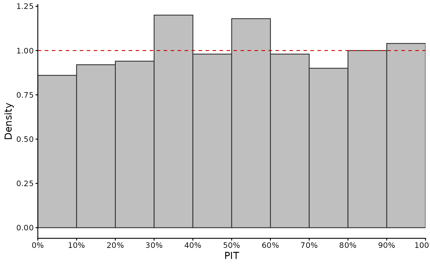
For calibrated continuous predictive distributions, PIT values evaluated over independent validation observations should be approximately uniformly distributed between zero and one. Individual PIT values do not have a preferred value; calibration is assessed from their distribution across observations, for example with gg_pit().

When cdf_at_obs is supplied, the values are returned after validation. This mode can be used with any continuous predictive distribution provided its CDF has already been evaluated at each corresponding observation.

Alternatively, obs, pred, and predictive_sd can be supplied together. In this case, normal predictive distributions are assumed and PIT values are calculated as

$$ u_i = \Phi\left( \frac{obs_i-pred_i}{\sigma_i} \right), $$

where $\Phi$ is the standard normal CDF and $\sigma_i$ is the predictive standard deviation.

A uniform PIT distribution is consistent with probabilistic calibration. Systematic departures from uniformity can indicate misspecification of the predictive distributions. For example, U-shaped PIT histograms are commonly associated with underdispersed predictive distributions, hump-shaped histograms with overdispersed distributions, and asymmetric PIT histograms with systematic bias. These patterns are diagnostic rather than unique and should be interpreted together with other validation measures.

PIT uniformity assesses the predictive distributions collectively and does not by itself establish that every aspect of conditional calibration is correct. Calibration should therefore generally be evaluated using complementary diagnostics such as gg_qcp(), gg_coverage(), and proper scoring rules.

The usual uniformity interpretation applies directly to continuous predictive distributions. For discrete distributions or finite predictive ensembles, ordinary PIT values are discrete; randomized PIT or rank-based diagnostics are more appropriate.

With predictive samples, pit() returns the fraction of draws less than or equal to each observation (including ties). This empirical CDF requires no normal assumption. With na.rm = TRUE, rows missing obs or any draw are removed together; with na.rm = FALSE, an incomplete row makes all returned PIT values NA, retaining the original observation-vector length.

References

Gneiting, T., Balabdaoui, F. and Raftery, A. E. (2007). Probabilistic forecasts, calibration and sharpness. Journal of the Royal Statistical Society: Series B, 69, 243-268. doi:10.1111/j.1467-9868.2007.00587.x

Schmidinger, J. and Heuvelink, G. B. M. (2023). Validation of uncertainty predictions in digital soil mapping. Geoderma, 437, 116585. doi:10.1016/j.geoderma.2023.116585

Examples

# PIT values from CDF values calculated elsewhere
cdf_values <- stats::pnorm(c(-1, 0, 1))
pit(cdf_values)
#> [1] 0.1586553 0.5000000 0.8413447

# Calculate PIT directly for normal predictive distributions
set.seed(123)

n <- 500
pred <- seq(0, 10, length.out = n)
predictive_sd <- rep(1, n)
obs <- stats::rnorm(n, mean = pred, sd = predictive_sd)

pit_values <- pit(
  obs = obs,
  pred = pred,
  predictive_sd = predictive_sd
)

gg_pit(pit_values)

pit(obs = 1:3, distribution = cbind(0:2, 1:3, 2:4))
#> [1] 0.6666667 0.6666667 0.6666667