
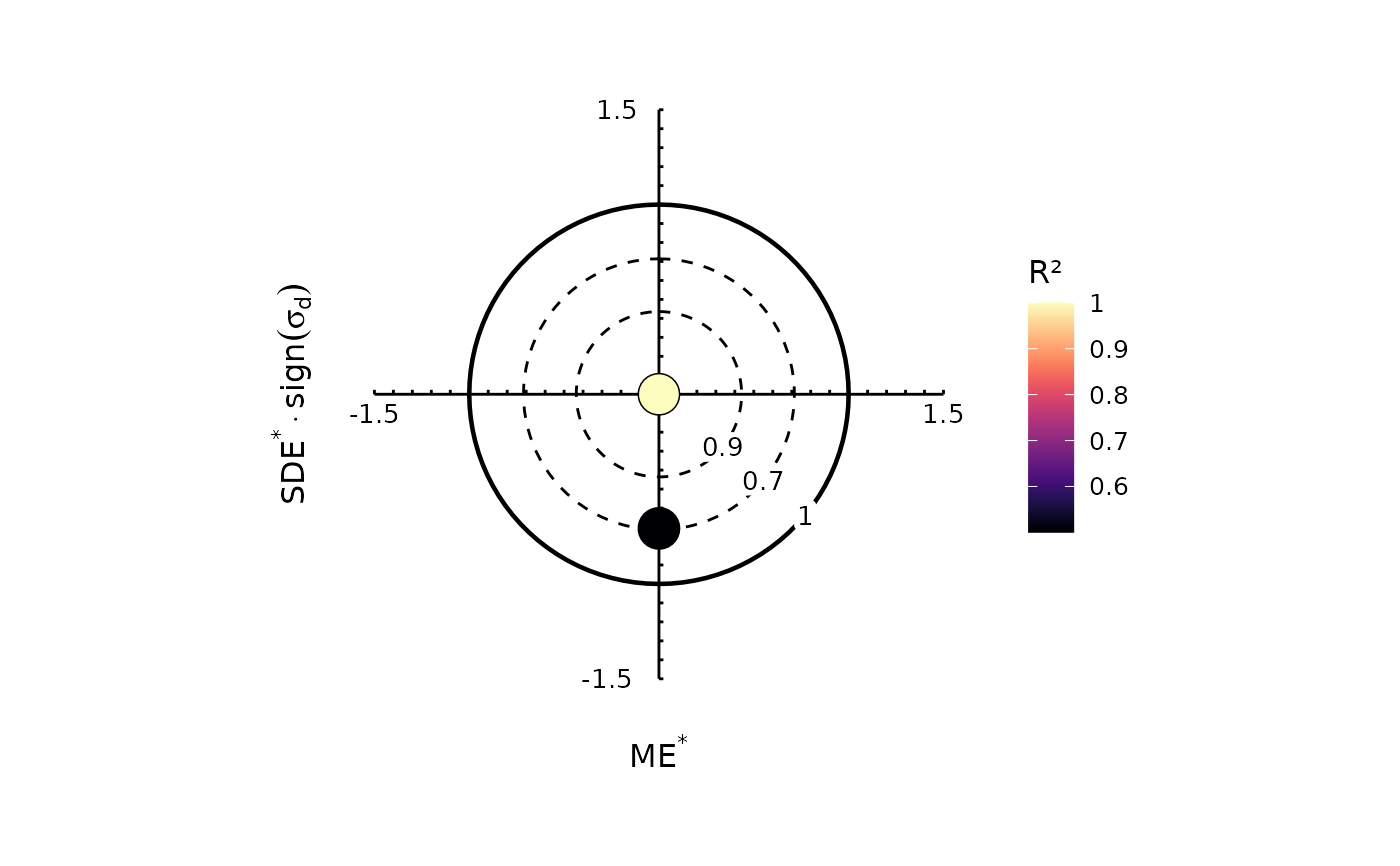
Creates a target diagram comparing quantitative prediction models with an observation vector. The horizontal coordinate is the signed standardized unbiased root mean square difference and the vertical coordinate is normalized mean error. The dashed inner circles delimit regions implying minimum Pearson correlation levels, whereas the solid unit circle provides an RMSE* reference.
Usage
gg_target(
  mods,
  obs,
  colorval = NULL,
  colorval.name = NULL,
  colour_by = c("efficiency", "model", "correlation", "r2"),
  axis_begin = -1.5,
  axis_end = 1.5,
  by = 0.1,
  label = FALSE,
  point_size = 7,
  label_size = 4,
  na.rm = TRUE,
  legend = TRUE,
  reference = TRUE
)
Arguments
- mods
Numeric vector, list of numeric vectors, or numeric matrix/data frame with one model per column. Rows match
obsin order. Supplied model names must be unique; missing names are generated.- obs
A numeric observation vector.
- colorval
Optional finite numeric vector with one value per model, in model order. When supplied, it overrides the continuous metric selected by
colour_by.- colorval.name
Optional point-colour legend title. The title can also be replaced afterwards with
labs(fill = ...).- colour_by
Character string defining point colouring.
"efficiency"uses uppercase R-squared / NSE / MEC and is the default;"model"gives every model a categorical colour and model-name legend;"correlation"uses Pearson correlation; and"r2"uses squared Pearson correlation.- axis_begin
Lower endpoint of both manually drawn reference axes. Defaults to -1.5.
- axis_end
Upper endpoint of both manually drawn reference axes. Defaults to 1.5.
- by
Spacing between manually drawn reference-axis ticks.
- label
Logical; draw model names beside points using
ggrepel?- point_size
Numeric point size.
- label_size
Numeric size of model labels.
- na.rm
Logical; remove incomplete observation-prediction pairs separately for each model? If
FALSE, missing pairs cause an error because diagram coordinates cannot be calculated. The default isTRUE.- legend
Logical; show the point-colour legend?
- reference
Logical; draw the target-diagram reference circles and their labels? The dashed inner circles indicate regions implying minimum Pearson correlation levels, whereas the solid unit circle represents the RMSE* = 1 reference.
Value
A ggplot2 object that can be extended with ordinary ggplot2 layers,
scales, labels, themes, and coordinates.
Details
The default geometry follows Wadoux, Walvoort, and Brus (2022). By default, points are coloured by the model-efficiency coefficient R-squared, equivalent to NSE and MEC in modelskill.
Missing pairs are removed separately per model when na.rm = TRUE.
Two complete pairs with non-zero observation standard deviation are required.
The default point-colour variable is the uppercase modelskill R2(), which
is equivalent to NSE and MEC. This should not be confused with lowercase
r2(), which is squared Pearson correlation.
The function returns an ordinary ggplot2 object. Styling that belongs to the
ggplot2 ecosystem can therefore be applied after the function call. Use
labs() for titles, theme() for typography and legend placement, and
scale_fill_*() to replace the point-colour scale.
The axis arguments control the manually drawn target-diagram reference axes rather than clipping limits. Models outside those reference axes remain visible. Equal coordinate scaling is retained so that the reference circles remain circular.
Coordinates and labels
The horizontal coordinate is signed_sde and the vertical coordinate is
nME. To retain the presentation of the original implementation, the
displayed horizontal title is ME* and the displayed vertical title is
SDE* multiplied by the sign of the standard-deviation difference.
Interpretation
The target diagram combines the solar error decomposition
$$\mathrm{RMSE}^{*2} = \mathrm{ME}^{*2} + \mathrm{SDE}^{*2}$$
with the sign of the prediction-versus-observation standard-deviation
difference. The signed SDE coordinate distinguishes predictions with less
variation than observations from predictions with greater variation; the
mean-error coordinate distinguishes overprediction (negative ME*) from
underprediction (positive ME*) under the obs - pred convention. The
distance to the origin is RMSE normalized by the population-moment
observation standard deviation, so points near the origin are preferred.
The reference circles have two distinct interpretations. The dashed inner circles correspond to correlation lower-bound regions, with radius \(\sqrt{1-r^2}\) for the displayed Pearson correlation threshold. The solid unit circle instead represents the RMSE* = 1 reference. A point near the origin is both close in mean and in spread/pattern; a point displaced along the mean-error direction is chiefly biased; and a point displaced along the signed-SDE direction chiefly differs in variability or pattern. The displayed titles intentionally retain the original implementation's visual orientation; use the coordinate definitions above when interpreting position.
ggplot2 customization
Arguments that change the statistical content or core target-diagram
construction are exposed directly by gg_target(). Ordinary appearance is
intentionally left to ggplot2. For example, users can add labs(), theme(),
a replacement scale_fill_*(), or a replacement coord_fixed().
References
Wadoux, A. M. J.-C., Walvoort, D. J. J., and Brus, D. J. (2022). An integrated approach for the evaluation of quantitative soil maps through Taylor and solar diagrams. Geoderma, 405, 115332. doi:10.1016/j.geoderma.2021.115332
Jolliff, J. K., Kindle, J. C., Shulman, I., Penta, B., Friedrichs, M. A. M., Helber, R., and Arnone, R. A. (2009). Summary diagrams for coupled hydrodynamic-ecosystem model skill assessment. Journal of Marine Systems, 76, 64-82. doi:10.1016/j.jmarsys.2008.05.014
Examples
obs <- c(1, 2, 3, 4, 5)
mods <- list(perfect = obs, biased = obs + 1)
# Default: point colour represents R-squared / NSE / MEC.
gg_target(mods, obs)
 # Give every model a categorical colour and a model-name legend.
p_models <- gg_target(mods, obs, colour_by = "model")
# Write model names directly beside points.
p_labels <- gg_target(mods, obs, label = TRUE)
# Standard ggplot2 customization.
p_custom <- gg_target(mods, obs) +
ggplot2::labs(title = "Model performance") +
ggplot2::theme(legend.position = "bottom")
# Print p_models, p_labels or p_custom to display a variant.
# Give every model a categorical colour and a model-name legend.
p_models <- gg_target(mods, obs, colour_by = "model")
# Write model names directly beside points.
p_labels <- gg_target(mods, obs, label = TRUE)
# Standard ggplot2 customization.
p_custom <- gg_target(mods, obs) +
ggplot2::labs(title = "Model performance") +
ggplot2::theme(legend.position = "bottom")
# Print p_models, p_labels or p_custom to display a variant.