Assessing and Visualising the Performance of Prediction Models • modelskill

Last update: 2026-09-09

Alexandre M.J.-C. Wadoux

About

modelskill is an R package for the evaluation of continuous predictions and their quantified uncertainty.

It can be used with predictions from machine-learning, statistical, geostatistical, physical, and process-based models. The package evaluates the predictions themselves rather than the algorithm that produced them.

modelskill brings together three complementary components:

prediction performance metrics, from RMSE and bias to correlation, agreement, and model efficiency;
predictive-uncertainty diagnostics, for prediction intervals, quantiles, and full predictive distributions;
summary diagrams and diagnostic plots, including solar, target, Taylor, coverage, PIT, and quantile-calibration plots.

All plotting functions return standard ggplot2 objects and can therefore be customised with the usual ggplot2 syntax.

Citation

If you use modelskill in your work, please cite the package as:

Wadoux, A.M.J.-C. (2026). modelskill: Assessing and Visualising the Performance of Prediction Models. R package version 0.1.0. https://github.com/AlexandreWadoux/modelskill

BibTeX

@Manual{wadoux2026modelskill,
  title  = {modelskill: Assessing and Visualising the Performance of Prediction Models},
  author = {Wadoux, A.M.J.-C.},
  year   = {2026},
  note   = {R package version 0.1.0},
  url    = {https://github.com/AlexandreWadoux/modelskill}
}

The citation can also be retrieved directly from R with:

citation("modelskill")

Documentation

Three tutorials cover the main functionality of the package:

Prediction performance metrics
Evaluate bias, error magnitude, association, agreement, efficiency, relative error, and specialised prediction losses.
Predictive-uncertainty evaluation
Validate prediction intervals, predictive standard deviations, quantiles, predictive samples, and full predictive distributions.
Summary diagrams and diagnostic plots
Compare models visually with solar, target, and Taylor diagrams and learn how to customise them with ggplot2.

Full function documentation is available on the modelskill website.

Main functionality

Task	Main functions
Prediction performance	`model_metrics()`, `rmse()`, `mae()`, `bias()`, `correlation()`, `r2()`, `R2()`, `ccc()`, `kge()`
Predictive uncertainty	`uncertainty_metrics()`, `picp()`, `interval_width()`, `interval_score()`, `qcp()`, `pit()`, `crps()`
Uncertainty diagnostics	`gg_coverage()`, `gg_qcp()`, `gg_pit()`
Summary diagrams	`gg_solar()`, `gg_target()`, `gg_taylor()`

Installation

Install the development version from GitHub:

install.packages("remotes")
remotes::install_github("AlexandreWadoux/modelskill")

Then load the package:

library(modelskill)

Development status: modelskill is under active development and has not yet been submitted to CRAN.

Validation statistics

Suppose several models have predicted the same observations:

library(modelskill)

set.seed(123)

obs <- seq(0, 10, length.out = 100) +
  rnorm(100, sd = 1)

models <- list(
  Good = obs + rnorm(100, sd = 0.5),
  Biased = obs + 1,
  Noisy = obs + rnorm(100, sd = 2)
)

Evaluate prediction performance

Evaluate all models simultaneously:

model_metrics(models, obs, digits = 3)

Or calculate individual statistics:

rmse(obs, models$Good)

bias(obs, models$Biased)

correlation(obs, models$Good)

R2(obs, models$Good)

A central principle of modelskill is that different metrics describe different aspects of prediction performance.

For example, lowercase r2() is squared Pearson correlation, whereas uppercase R2() is the model-efficiency coefficient:

r2(obs, models$Biased)

R2(obs, models$Biased)

A systematically biased prediction can have r2 = 1 while having imperfect model efficiency.

See the prediction-performance tutorial for interpretation of the available metrics.

Uncertainty statistics

modelskill evaluates quantified predictive uncertainty represented as:

predictive means and standard deviations;
full predictive distributions.

Prediction intervals

For example, evaluate a 95% prediction interval:

pred <- models$Good
predictive_sd <- rep(1, length(obs))

lower95 <- pred + qnorm(0.025) * predictive_sd
upper95 <- pred + qnorm(0.975) * predictive_sd

uncertainty_metrics(
  obs,
  lower = lower95,
  upper = upper95,
  level = 0.95
)

The output includes prediction interval coverage, coverage error, interval width, and interval score.

Predictive mean and standard deviation

A normal predictive distribution specified by its mean and standard deviation can be evaluated directly with CRPS:

crps(
  obs,
  pred = pred,
  predictive_sd = predictive_sd
)

Calibration across several interval levels can be visualised with:

gg_coverage(
  obs,
  pred = pred,
  predictive_sd = predictive_sd
)

Predictive samples

When complete predictive samples are available, retain the full distributions:

set.seed(456)

predictive_samples <- sapply(
  seq_len(200),
  function(i) {
    rnorm(
      length(obs),
      mean = pred,
      sd = predictive_sd
    )
  }
)

crps(
  obs,
  distribution = predictive_samples
)

See the predictive-uncertainty tutorial for prediction intervals, QCP, PIT, CRPS, predictive samples, and scoring rules.

Graphical summaries

modelskill provides solar, target, and Taylor diagrams for comparing several aspects of model performance simultaneously.

gg_solar(models, obs, label = TRUE)

gg_target(models, obs, label = TRUE)

gg_taylor(models, obs, label = TRUE)

Graphical model evaluation

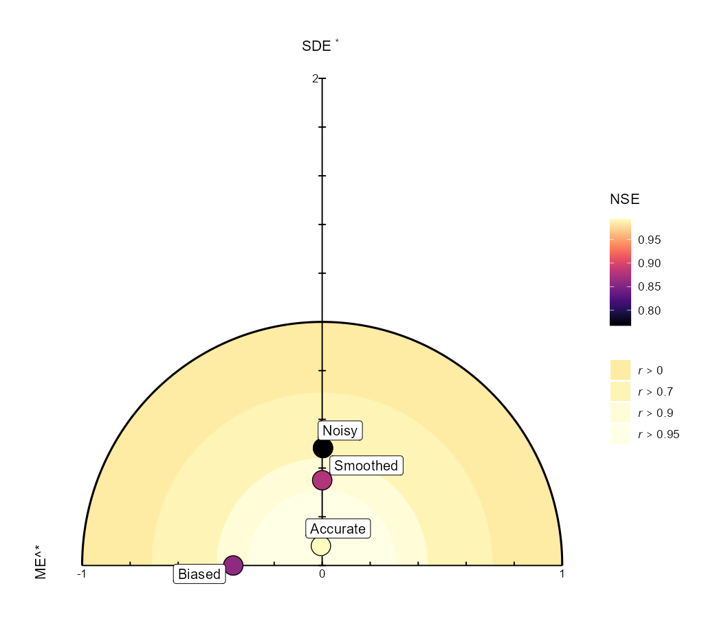
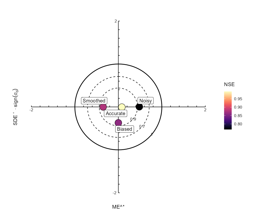
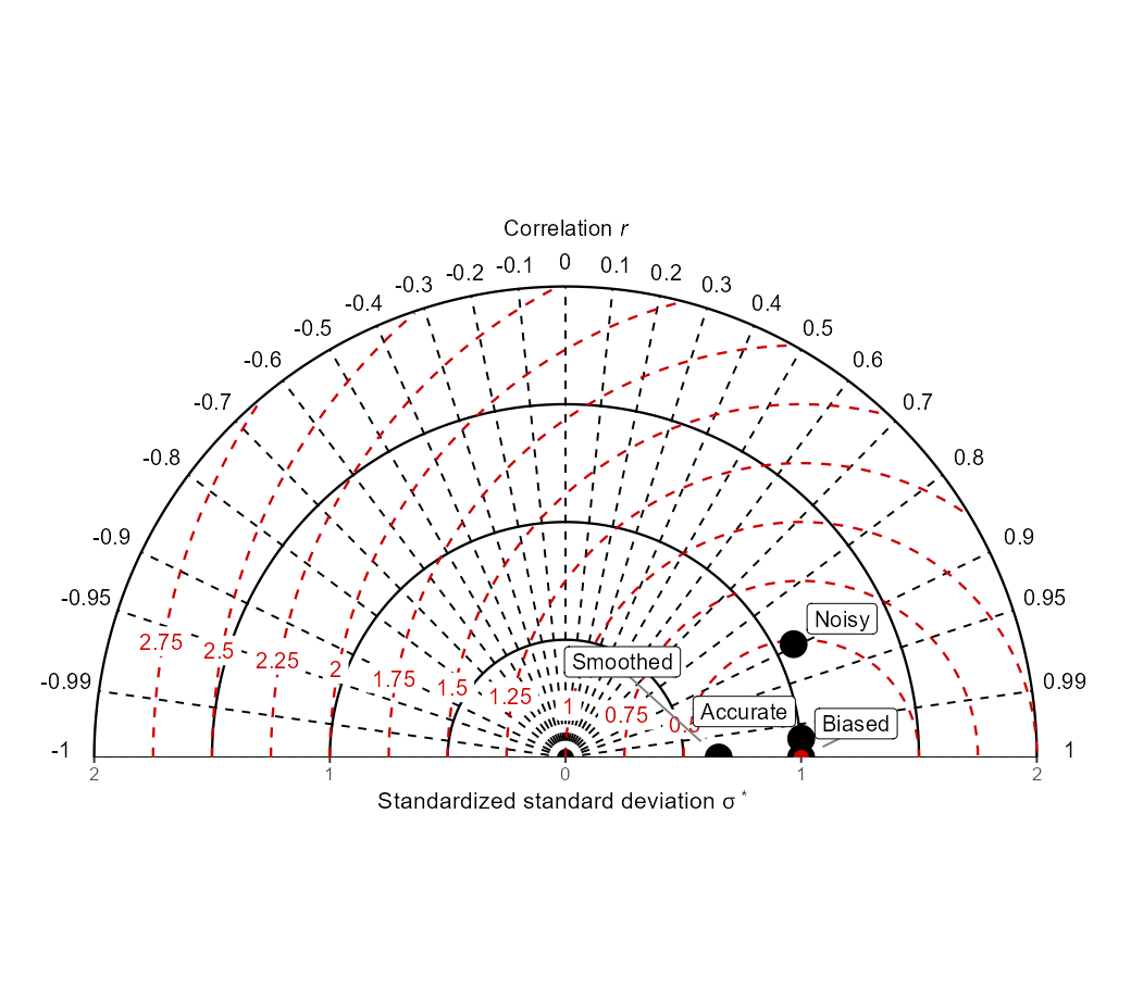
Solar diagram Target diagram Taylor diagram

The three diagrams provide complementary information:

the solar diagram combines mean error, centred error, total error, and additional performance information;
the target diagram additionally distinguishes whether predictions have less or more variability than the observations;
the Taylor diagram focuses on correlation, relative variability, and centred error.

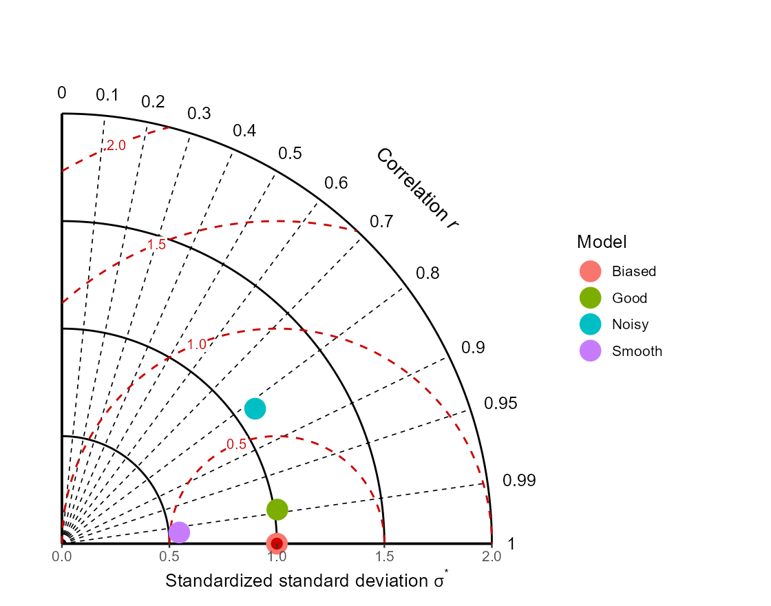
The Taylor diagram can also be displayed using only positive correlations:

gg_taylor(
  models,
  obs,
  legend = TRUE,
  half = TRUE
)

This half-diagram view is useful when negative correlations are not relevant to the comparison, giving the positive-correlation region more visual space.

Half Taylor diagram showing positive correlations only

See the summary-diagram tutorial for interpretation and additional options.

Customising plots

All plotting functions return ordinary ggplot2 objects.

For example:

gg_solar(
  models,
  obs,
  colour_by = "model"
) +
  ggplot2::labs(
    title = "Model comparison"
  ) +
  ggplot2::theme(
    legend.position = "bottom"
  )

The same principle applies to solar, target, Taylor, coverage, PIT, and QCP plots.

Scientific basis

The solar and Taylor diagram implementations build on:

Wadoux, A. M. J.-C., Walvoort, D. J. J. & Brus, D. J. (2022).
An integrated approach for the evaluation of quantitative soil maps through Taylor and solar diagrams.
Geoderma, 405, 115332.
https://doi.org/10.1016/j.geoderma.2021.115332

The Taylor diagram was originally introduced by:

Taylor, K. E. (2001).
Summarizing multiple aspects of model performance in a single diagram.
Journal of Geophysical Research: Atmospheres, 106, 7183–7192.
https://doi.org/10.1029/2000JD900719

The target diagram follows:

Jolliff, J. K., Kindle, J. C., Shulman, I., Penta, B., Friedrichs, M. A. M., Helber, R. & Arnone, R. A. (2009).
Summary diagrams for coupled hydrodynamic-ecosystem model skill assessment.
Journal of Marine Systems, 76, 64–82.
https://doi.org/10.1016/j.jmarsys.2008.05.014

Predictive-uncertainty validation is informed by:

Schmidinger, J. & Heuvelink, G. B. M. (2023).
Validation of uncertainty predictions in digital soil mapping.
Geoderma, 437, 116585.
https://doi.org/10.1016/j.geoderma.2023.116585

Getting help

Function documentation is available directly in R:

?model_metrics
?uncertainty_metrics
?gg_solar
?gg_target
?gg_taylor

Bug reports and feature requests can be submitted through the GitHub issue tracker.

Author and licence

Alexandre M.J.-C. Wadoux
Author, maintainer, and copyright holder

modelskill is released under the MIT License.